Random Forest

Random forest is a classic machine learning ensemble method that is a popular choice in data science.

An ensemble method is a machine learning model that is formed by a combination of less complex models. In this case, our Random Forest is made up of combinations of Decision Tree classifiers.

How this work is through a technique called bagging. In bagging, each Decision Tree trains on a different subsample of the training data and then their predictions are combined for a final output.

The cool thing about ensembling a lot of decision trees is that the final prediction is much better than each individual classifier because they pick up on different trends in the data.

In this post we will take a look at the Random Forest Classifier included in the Scikit Learn library.

Getting our data

Before we can train a Random Forest Classifier we need to get some data to play with.

We will be taking a look at some data from the UCI machine learning repository. The dataset we will use is the Balance Scale Data Set. You can learn more about the dataset here.

Dataset Overview

The balance scale dataset contains information on different weight and distances used on a scale to determine if the scale tipped to the left(L), right(R), or it was balanced(B).

The class name informs us the direction that the scale was pointing towards and it will be the target variable for our analysis.

So for example, if we have a row of data that contains (left_weight: 1, left_distance:1, right_weight:1, right_distance:2, class_name: R).

It would mean that in a single scale observation, a 1 unit weight was place on left side at 1 unit distance from the mid point and a 1 unit weight was placed on the right side at 2 unit weights from the mid point and the scale tilted to the right(R) side.

Here are the possible data columns and values:

1. Class Name: 3 (L, B, R)
2. Left-Weight: 5 (1, 2, 3, 4, 5)
3. Left-Distance: 5 (1, 2, 3, 4, 5)
4. Right-Weight: 5 (1, 2, 3, 4, 5)
5. Right-Distance: 5 (1, 2, 3, 4, 5)

Exploratory Data Analysis

It’s finally time to take a look at our data. Let’s import pandas and read the data from the UCI website.

import pandas as pd
column_names = ['class_name', 'left_weight', 'left_distance', 'right_weight', 'right_distance']
df = pd.read_csv('https://archive.ics.uci.edu/ml/machine-learning-databases/balance-scale/balance-scale.data',
header=None,
names=column_names
)

After loading our dataset, let’s take a look at our data by accessing the first few items.

df.head()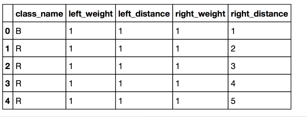

Our output shows that our data looks good and that it imported correctly.

Now, let’s get some additional information on the data.

df.info()

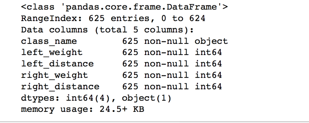
Our output shows that we have 625 data entries and there are no empty or null values. Nice!

df['class_name'].value_counts()

Value_counts shows us that there are 288 targets of L and R each and then there are 49 classes of B(balanced) classes. This dataset seems to be fairly balanced.

Next, let’s split our data into features and targets.

data_cols = ['left_weight', 'right_weight', 'left_distance', 'right_distance']
target_cols = ['class_name']

X = df[data_cols]
y = df[target_cols]

X will hold onto the data for our feature columns and y will hold our target data.

Next, let’s break up our features X and targets y into train and test sets. We need separate sets of data so that our model can be trained on the training set and then tested on the test set. If we only had one set of data, then there will be no way to check how well our model is performing.

from sklearn.model_selection import train_test_split

X_train, X_test, y_train, y_test = train_test_split(X, y, test_size=0.3, random_state=42)

In this instance, I used train_test_split function from Scikit Learn to break up our datasets. A test_set of 0.3 will give us 30% of the data in x_test/y_test while x_train/y_train holds 70% of the data.

We are finally ready to train our first random forest model on our dataset.

from sklearn.ensemble import RandomForestClassifier
from sklearn.metrics import accuracy_score

model = RandomForestClassifier()
model.fit(X_train, y_train)
y_predict = model.predict(X_test)

accuracy_score(y_test.values, y_predict)

After creating our random forest classifier, we fit the model with its default parameters on our X_train and y_train.

We will be determining the performance of our model with accuracy_score. Accuracy is a metric that determines the fraction of true positives and true negatives out of all predictions.

Basically, accuracy is just the number of correct predictions divided by the number of total predictions.

We will be getting our accuracy score by comparing the predicted values(y_predict) versus the real values(y_test.values)

With our minimum effort model, we were able to get 79.3% of the predictions correctly. Next, let’s try to do some feature engineering on our data to see if we can get a better performing model.

Feature Engineering

Feature engineering is the process of taking our feature data and combining them in different ways to create new features that might help our model generalize on the target variable.

Attempt #1

So in our dataset, we have a bunch of weights and lengths that describe weights placed on left and right sides of our scale. Intuition tells me that we could try to get a product(multiplication) of the weight and lengths for a new feature. Let’s try it.

I’ll call these new features ‘left_cross’ and ‘right_cross’.

df['left_cross'] = df['left_distance'] * df['left_weight']
df['right_cross'] = df['right_distance'] * df['right_weight']

Let’s take a look at how these new features affected our model’s ability to predict the target variable.

new_data_cols = ['left_weight', 'right_weight', 'left_distance', 'right_distance', 'left_cross', 'right_cross']
new_target_cols = ['class_name']

X = df[new_data_cols]
y = df[new_target_cols]
X_train, X_test, y_train, y_test = train_test_split(X, y, test_size=0.3, random_state=42)

forest = RandomForestClassifier()
forest.fit(X_train, y_train)
y_predict = forest.predict(X_test)
accuracy_score(y_test, y_predict)

After adding the left and right products into our feature set, we trained a new random forest on the features. The accuracy shows that our model has improved to a healthy 89.4%.

Attempt #2

Although 89.4% is pretty good, let’s try one more attempt at feature engineering to squeeze everything out of our data.

Another intuition tells me that getting a ratio between the products of the left and right sides might be useful. Since a scale is just comparing the stuff on the left side to the right side.

We will call this new feature ‘left_right_ratio’.

new_data_cols = ['left_weight', 'right_weight', 'left_distance', 'right_distance', 'left_cross', 'right_cross', 'left_right_ratio']
new_target_cols = ['class_name']

df['left_right_ratio'] = df['left_cross']/df['right_cross']

df.head()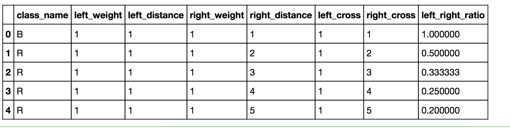

After our last attempt at feature engineering, this is how our features dataset looks.

Finally, it’s time for our model to train on our new and improved dataset.

X = df[new_data_cols]
y = df[new_target_cols]
X_train, X_test, y_train, y_test = train_test_split(X, y, test_size=0.3, random_state=42)

new_forest = RandomForestClassifier()
new_forest.fit(X_train, y_train)

y_predict = new_forest.predict(X_test)
accuracy_score(y_test, y_predict)

Our accuracy shows 98.9% of the predictions were correct! Our work on feature engineering looks to have paid off.

Let’s show how important each feature was to helping our model perform.

features_dict = {}
for i in range(len(new_forest.feature_importances_)):
    features_dict[new_data_cols[i]] = new_forest.feature_importances_[i]
sorted(features_dict.items(), key=lambda x:x[1], reverse=True)

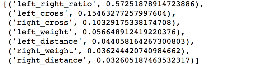
Feature importances show that left_right_ratio is by far the most important feature.

Our last attempt at improving our accuracy will be with hyperparameter tuning.

Hyperparameter Tuning With Grid Search

Hyperparameter tuning is essentially making small changes to our Random Forest model so that it can perform to its capabilities.

We will use GridSearchCV which will help us with tuning. GridSearchCV will try every combination of hyperparameters on our Random Forest that we specify and keep track of which ones perform best.

from sklearn.model_selection import GridSearchCV

gridsearch_forest = RandomForestClassifier()

params = {
    "n_estimators": [100, 300, 500],
    "max_depth": [5,8,15],
    "min_samples_leaf" : [1, 2, 4]
}

clf = GridSearchCV(gridsearch_forest, param_grid=params, cv=5 )
clf.fit(X,y)

In this example, we will only be grid searching ‘n_estimators’, ‘max_depth’, and ‘min_samples_leaf’.

n_estimators is the number of decision trees to use for our random forest model.

max_depth is the maximum depth of each decision tree.

min_samples_leaf is the minimum number of samples required to be at a leaf node in each decision tree.

*It should be noted that grid search is a computationally intensive task on large data sets and that n_estimators could be a feature that is low priority for grid searching, since models with more tree estimators tend to perform better. *

 

After fitting our grid search object on our dataset, we can take a look at the best performing hyperparameters and how well that model scores.

clf.best_params_

It looks like the performing model had a max_depth of 5, min_samples_leaf of 1 and n_estimators of 100.

clf.best_score_

With that model, we were able to predict 100 percent of the time whether the scale was leaning left, right or balanced based on the weights placed on the scale.

100% accuracy might seem too good to be true at first glance, but in these circumstances, this data can be backed by physics and the balancing of forces and torques.

So after some further inspection, our model looks to be doing pretty well.

Conclusion

In this post, we were able to take a look at the balance scale dataset from the UCI machine learning repository.

We went through exploratory data analysis, feature engineering, modeling with Random Forest, and then hyperparameter tuning on our model.

I hope this helped you with understanding machine learning with Random Forest and Scikit Learn.

Please let me know if you have any questions 🙂